Creating Riemann's Minimal Surface 3D model in python

f:id:asahidari:20200509112713p:plain

Overview

When Searching for Riemann's minimal surface, you can find many drawings generated in Mathematica. But it seems difficult to find the way to create the surface in another environments. So I tried to make another example,using python. (Octave or MATLAB may be possible to do the same thing.)

Parametric equations for the Riemann's Minimal Surface

I found an article about parametric equations to generate a fundamental piece of the surface, the title of the writing is 'The Riemann Minumal Examples'*1. In this document, mathematical equations and functions to calculate X,Y,Z values of the surface are written in chapter 4.2.1 'Parametarizing the surface with Mathematica'.

Using sympy's elliptic integral functions

In the document, you will find elliptic integral functions (ellipticF, ellipticE) to get X, Y, Z values. In python, 'sympy'*2 has the functions(elliptic_f, elliptic_e), and it also offers plotting views(, using matplotlib as a backend).

Creating a fundamental piece of Riemann's minimal surface

Following the paper, I wrote the functions in python.

import sympy as sp
from sympy import symbols, re, im, I
from sympy.functions.special.elliptic_integrals import elliptic_f, elliptic_e

s_ = 2.0
e_ = 0.01 # <- Easy to connect with the rotated surface when exported in STL format

# symbols
r, t = symbols('r t')
s, z, a, e = symbols('s z a e')

# mobius transformation
f = (-a**2 * (1.+e**2) * (-1.+z) - 2*a * (-3.+e**2) * z - (1.+e**2) * (1.+z) \
     + sp.sqrt(4 * (-1.+a)**2 * e**2 + (1.+a)**2 * (-1.+e**2)**2) * (1.+a*(-1.+z)+z)) \
    * (2 * sp.sqrt(4 * (-1.+a)**2 * e**2 + (1.+a)**2 * (-1.+e**2)**2) \
       -2 * ( (1.+a) * (-1.+e**2) - 2 * (-1.+a) * z ))

# three coordinate functions
x1 = (1./sp.sqrt(s)) * ((sp.sqrt((-1.+z)/z)) * (sp.sqrt(z+s)) \
        + (1./sp.sqrt(1.+s)) * (2 * ((-1.-s) * elliptic_e(sp.asin(sp.sqrt(1.+(z/s))), (s/(1.+s))) \
        + elliptic_f(sp.asin(sp.sqrt(1.+(z/s))), (s/(1.+s))))))
x2 = -(sp.sqrt( (-1.+z)/(-s*z) )) * (sp.sqrt(s+z))
x3 = (-2./sp.sqrt(s)) * elliptic_f(sp.asin(sp.sqrt(s)/sp.sqrt(s+z)), ((1.+s)/s))

# origin
v0_1 = -2 * sp.im ((1./sp.sqrt(-(1+s)*s))
        * ((-1.-s) * elliptic_e(sp.asin(sp.sqrt((1.+s)/s)), (s/(1.+s))) \
        + elliptic_f(sp.asin(sp.sqrt((1.+s)/s)), (s/(1.+s)))))
v0_2 = 0.0
v0_3 = -2 * sp.re((1./sp.sqrt(s)) * elliptic_f(sp.asin(sp.sqrt(s/(1.+s))), ((1.+s)/s)))

# plotting functions
psi_x = sp.re(x1) - (v0_1)
psi_y = sp.re(x2) - (v0_2)
psi_z = sp.re(x3) - (v0_3)
f_z = f.subs([(z, (r * sp.exp(I * sp.pi * t))), (a, s_), (e, e_)])

# XYZ values for surfaces
X = psi_x.subs([(s, s_), (z, f_z)])
Y = psi_y.subs([(s, s_), (z, f_z)])
Z = psi_z.subs([(s, s_), (z, f_z)])

After defining the equations, 3d plotting shows the piece in a graph view.

from sympy.plotting import plot3d_parametric_surface, plot3d_parametric_line

# plot 3d surface
p_ = plot3d_parametric_surface((X, Y, Z, (r, e_, 1.), (t, 0., 1.)), \
                               xlim=(-10, 10), ylim=(-10, 10), show=False)
p_.show()

The result is this.

f:id:asahidari:20200509114308p:plain

Rotating the piece around the center axis

After getting the fundamental piece, rotate it around the center axis and mirror it on the X or Y axis, to generate one 'step' of 'staircase' of the surface.

(To show the rotation-axis with the surface, I add a cross line to view the whole parts.)

# XYZ values for rotation axis parallel to y-axis
z_line = sp.sqrt(2.) * I 
Xl = psi_x.subs([(s, s_), (z, z_line)])
Yl = psi_y.subs([(s, s_), (z, z_line)]) + t*1
Zl = psi_z.subs([(s, s_), (z, z_line)])

# *** workaround for displaying in a moderate size box ***
# draw cross, not a line paralel to z axis
# due to plot3d_parametric_line's problem to plot constant functions -> https://github.com/sympy/sympy/issues/10529
zl_ = float(Zl)
Zl1_ = zl_ + t*0.5
Zl2_ = zl_ - t*0.5

# rotated around y-axis (, and later, need to shift to the rotation center point)
# when add 2*Xl or 2*Zl here, plotting will probably not work properly
Xr = -psi_x.subs([(s, s_), (z, f_z)]) #  + 2.*Xl
Yr = psi_y.subs([(s, s_), (z, f_z)])
Zr = -psi_z.subs([(s, s_), (z, f_z)]) #  + 2.*Zl

Then, plot them.

from sympy.plotting import plot3d_parametric_surface, plot3d_parametric_line

# plot 3d surface
p1 = plot3d_parametric_surface(X, Y, Z, (r, e_, 1.), (t, 0., 1.), \
                               xlim=(-10, 10), ylim=(-10, 10), show=False)
p2 = plot3d_parametric_line((Xl, Yl, Zl, (t, -8., 8.)), \
                            (Xl, Yl, Zl1_, (t, -8., 8.)), \
                            (Xl, Yl, Zl2_, (t, -8., 8.)), \
                            xlim=(-10, 10), ylim=(-10, 10), show=False)
p3 = plot3d_parametric_surface((Xr+2.*Xl, Yr, Zr+2*Zl, (r, e_, 1.), (t, 0., 1.)), \
                               xlim=(-10, 10), ylim=(-10, 10), show=False)
p4 = plot3d_parametric_surface((X, -Y, Z, (r, e_, 1.), (t, 0., 1.)), \
                               (Xr+2.*Xl, -Yr, Zr+2*Zl, (r, e_, 1.), (t, 0., 1.)), \
                               xlim=(-10, 10), ylim=(-10, 10), show=False)

p2.append(p1[0])

# this may requires huge time
p2.append(p3[0])
p2.append(p4[0])
p2.append(p4[1])

p2.show()

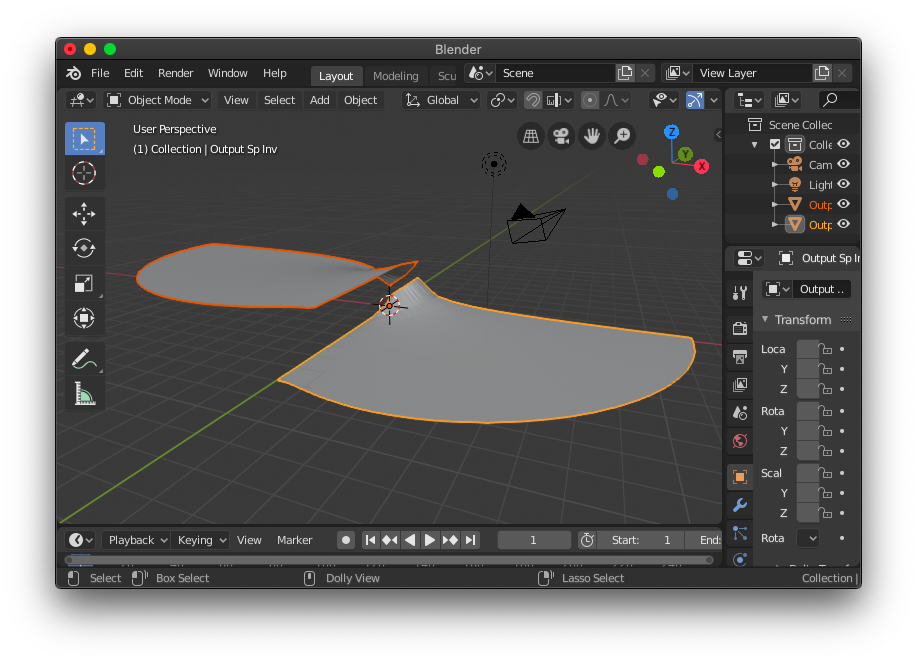
However, it requires long time to calculate and show all the results. So if you want to get the 'step' in short time, After exporting one or two pieces into STL files, rotate and mirror them by using other 3d softwares. Next image displays two pieces imoprted in Blender.

f:id:asahidari:20200509122031p:plain

Convert sympy symbols to numpy arrays

To export the 3d surface in STL format, you need to convert the sympy symbols to numpy arrays.

In this code, the symbols functions are once lambdified with 'mpmath' mode, and then changed to float arrays with fromnumpyfunc function. Because in 'numpy' mode, 'elliptic_f' and 'elliptic_e' functions cannot be recognized properly.

import numpy as np
from sympy.utilities.lambdify import lambdify

# parameters
r0 = np.linspace(e_, 1.0, 30)
t0 = np.linspace(0.0, 1.0, 30)
r_, t_ = np.meshgrid(r0, t0)
r_, t_ = r_.flatten(), t_.flatten()

X_ = lambdify((r, t), X, "mpmath")
Y_ = lambdify((r, t), Y, "mpmath")
Z_ = lambdify((r, t), Z, "mpmath")

X_npf = np.frompyfunc(X_, 2, 1)
Y_npf = np.frompyfunc(Y_, 2, 1)
Z_npf = np.frompyfunc(Z_, 2, 1)

X_np = X_npf(r_, t_).astype(float)
Y_np = Y_npf(r_, t_).astype(float)
Z_np = Z_npf(r_, t_).astype(float)

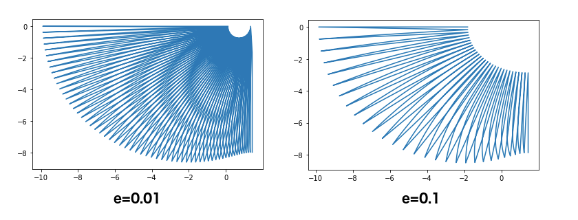
Before exporting the surface, I noted down about 'e' parameter.

Adjust 'e' parameters to modify the shape

In the first code, I assigned '0.01' to a parameter 'e' instead of default value '0.1' in the original article. Because when I use '0.1' to 'e', the inner circle is halved and opend, and the result makes it difficult to connect the original piece with the rotated one around the 'neck' part. (I'm not so familiar with elliptic integral functions, so please tell me if you know better options. ) Next code shows the difference.

import matplotlib.pyplot as plt

plt.plot(X_np, Y_np)

f:id:asahidari:20200509120720p:plain

Exporting to a STL file

After getting the surface graph, you can export the pieces into STL files by using surf2stl-python *3. (Probably, you can also get them by using numpy-stl *4.) This script triangulate the mesh. If you want quadified mesh, you can do it by using other 3d software tools. (For example, Blender offers the way to select Menu->Faces->Tri to Quad in Edit mode).

In this article, I exported the original piece and a rotated one.

from scipy.spatial import Delaunay
import surf2stl_python.surf2stl as s2s

delaunay_tri = Delaunay(np.array([r_, t_]).T)
s2s.tri_write('output_sp.stl', X_np, Y_np, Z_np, delaunay_tri)

Xr_ = lambdify((r, t), Xr+2*Xl, "mpmath")
Yr_ = lambdify((r, t), Yr, "mpmath")
Zr_ = lambdify((r, t), Zr+2*Zl, "mpmath")

Xr_npf = np.frompyfunc(Xr_, 2, 1)
Yr_npf = np.frompyfunc(Yr_, 2, 1)
Zr_npf = np.frompyfunc(Zr_, 2, 1)

Xr_np = Xr_npf(r_, t_).astype(float)
Yr_np = Yr_npf(r_, t_).astype(float)
Zr_np = Zr_npf(r_, t_).astype(float)

delaunay_tri = Delaunay(np.array([r_, t_]).T)
s2s.tri_write('output_sp_inv.stl', Xr_np, Yr_np, Zr_np, delaunay_tri)

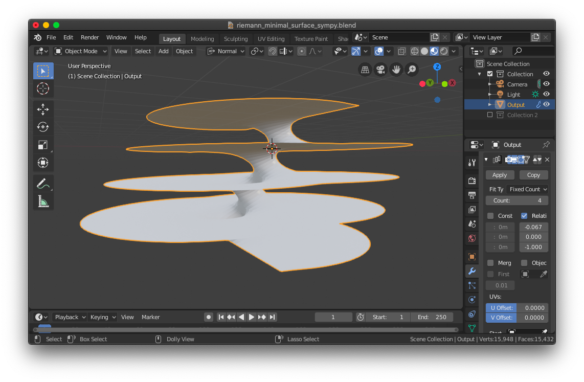
After some modifications (connecting the 'neck' parts, mirroring the connected one, copying the 'step', subdividing the surface, etc.), you'll get the 3d mesh of the Riemann's minimal surface. Here is the example in Blender.

f:id:asahidari:20200509122912p:plain